Introduction to AI
Module 2: A* examples
A* Examples
Sometimes it helps just to see a few extra examples of an algorithm!
Example 1
You are preparing to bake some birthday cupcakes but you need ingredients. Since your cake will be complicated, you need ingredients from two stores (Store A and Store B). Because of all the construction, your usual fastest routes are all messed up.
Map
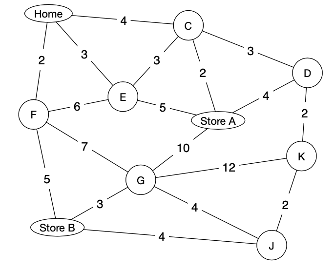
Distances
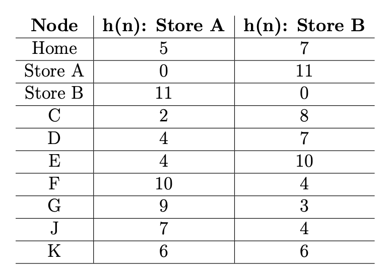
Search 1: Home to Store A
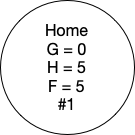
Step 1 is to add the initial state to the priority queue and then to grab it. This is shown below.
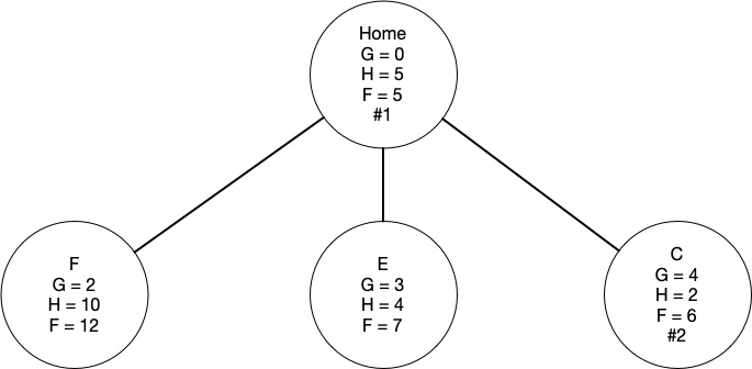
Since Home is not the goal node, we must add the children of home to the fringe. This adds F, E, and C as shown below. Note that we keep track of the heuristic values (f, g, and h) in the search tree. We choose C because its score (F = 6) is the lowest.
None of F, E, or C are the goal node so again we must add the children to the fringe. One note, C is able to reach E directly. We show this in the tree but do not connect it in since it is not a lower cost option than what is already in the tree (F = 7 in the direct route to E whereas F = 11 in the indirect route). Since Store A is the lowest cost option, we pull it from the queue and we are done with the first search.
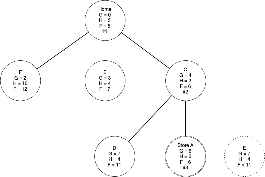
Note that the final path taken is the path from the goal to the root (then reversed): Home to C to Store A.
Search 2: Store A to Store B
Now we will search from Store A to Store B.
Step 1 is always to put the initial state into the queue.
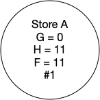
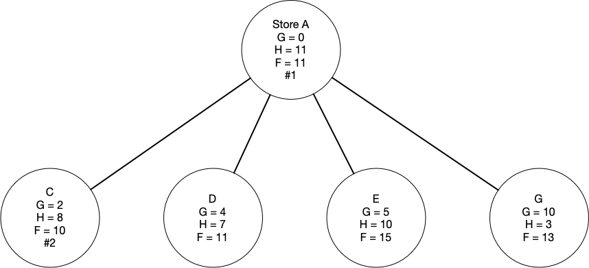
Since Store A is not our goal node, we need to add the children of Store A to the fringe.
Again, none of these are the goal node so we proceed to the lowest cost node. In this case, that is node C, which is marked as #2 here.
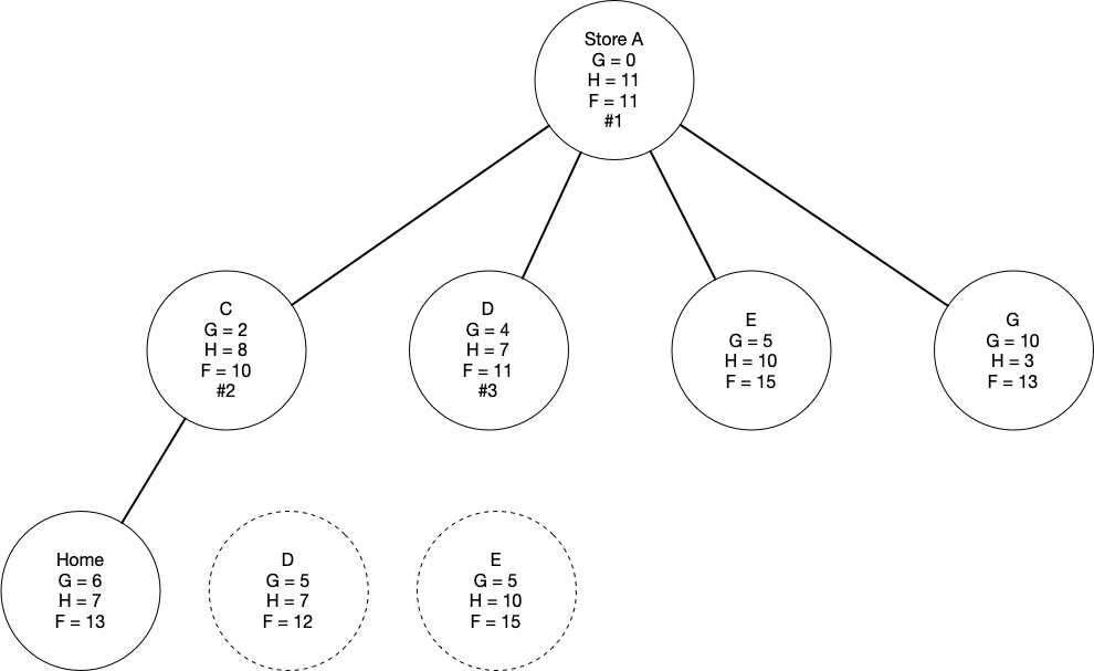
Note that for the step shown above, we considered both D an E but neither is lower-cost than their original entries in the priority queue and thus both are show dashed. Now time for a big important note: make sure you go to the lowest cost node in your fringe next! That is D here! (marked #3).
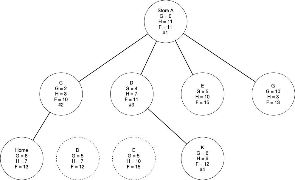
D has several paths but all of them except for K have already been explored. Thus only K is added to the fringe. Note that K is the lowest cost option and therefore becomes #4 in the search.
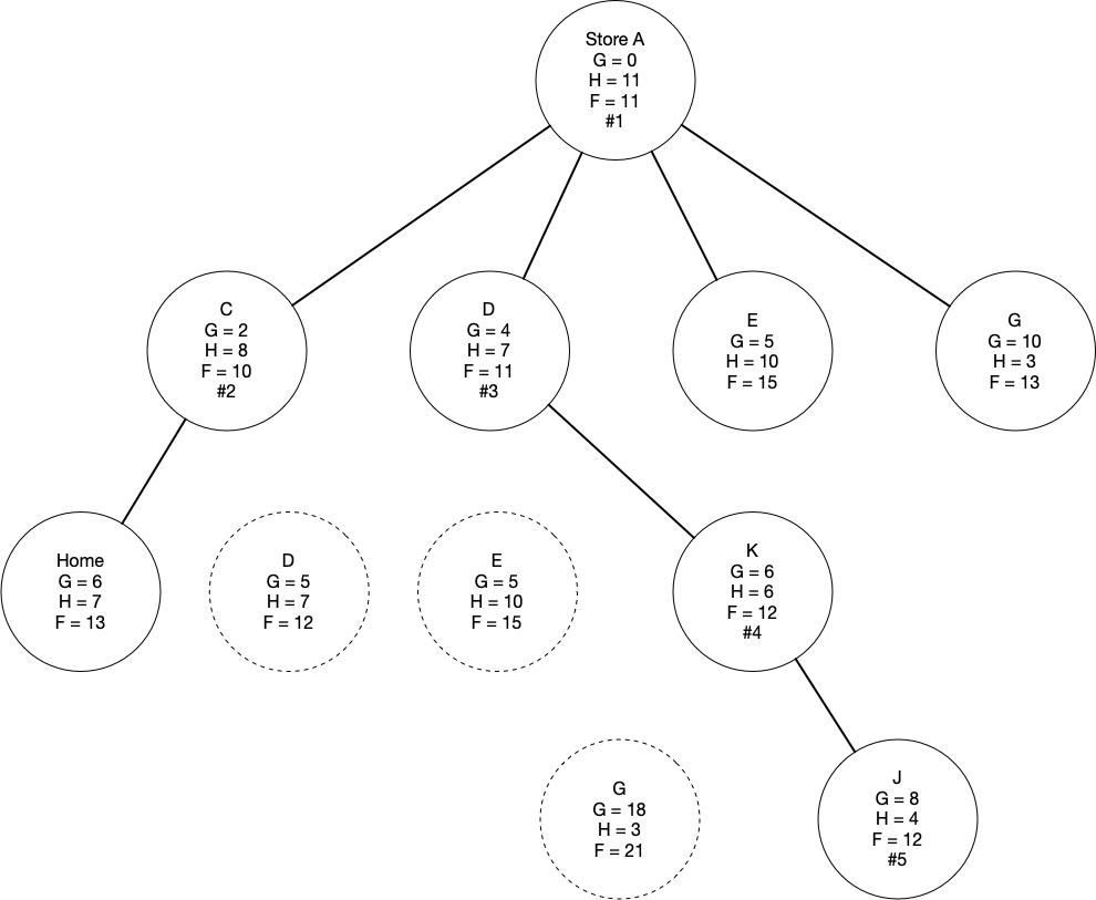
As before, K can visit several paths but G is higher cost and thus is not added. J is added and is now the lowest cost node in the fringe and becomes #5 in the search order.
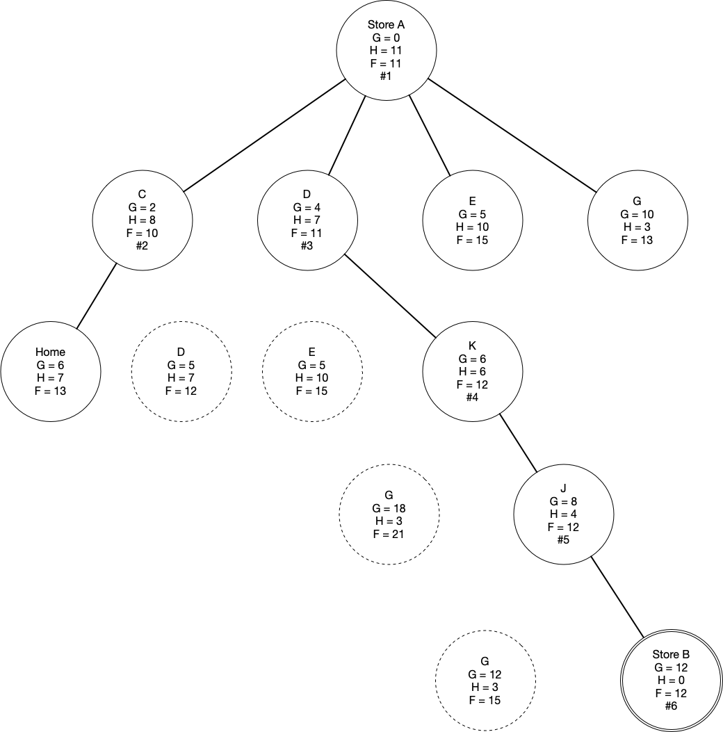
Finally, J can reach G again (but higher cost) and Store B, which is the goal and the lowest cost in the fringe. The search stops when we will the goal node from the fringe.
Note that the final path taken is the path from the goal to the root (then reversed). This means the final path does NOT include the detour to C that the search explored! The final path is Store A to D to K to J to Store B.